Download
1 / 47
480 likes | 885 Views
Aggregate Expenditure. Outline Components of aggregate expenditure Planned and unplanned expenditure The consumption function Imports and GDP Equilibrium expenditure The expenditure multiplier. Components of Aggregate Expenditure.
 orsin
orsin

E N D
Aggregate Expenditure • Outline • Components of aggregate expenditure • Planned and unplanned expenditure • The consumption function • Imports and GDP • Equilibrium expenditure • The expenditure multiplier
Components of Aggregate Expenditure • Recall from Chapter 5 that aggregate expenditure for final goods and services equals the sum of • Consumption expenditure, C • Investment, I • Government purchases of goods and services, G • Net exports, NX Thus:Aggregate expenditure = C + I + G + NX
Planned and Unplanned Expenditures Aggregate expenditure equals aggregate income and real GDP. But aggregate planned expenditure might not equal real GDP because firms can end up with larger or smaller inventories than they had intended.
Aesop’s Bottles B.C. 400 Investment Plans
Autonomous versus induced Expenditure • Autonomous expenditure: The components of aggregate expenditure that do not change when real GDP changes. • Induced expenditure: The components of aggregate expenditure that change when real GDP changes.
The Consumption Function The consumption function shows the relationship between consumption expenditure and disposable income, holding all other influences on influences on household spending behavior constant.
What is disposable income? • Disposable income is aggregate income (GDP) minus net taxes • Net taxes are taxes paid to government minus transfer payments received from government.
Source: Bureau of Economic Analysis
450 line Consumption (trillions of 2000dollars) Saving F Consumption function E D 6.0 Dissaving C Saving is zero B 2.0 A 2.0 6.0 10.0 Disposable income (trillions of 2000 dollars) (trillions of 2000 dollars)
Notice that autonomous consumption is given by point A. This is planned consumption expenditure when disposable income is zero ($1.5 trillion). This spending must be financed by past saving or by borrowing
Marginal Propensity to Consume (MPC) The marginal propensity to consume (MPC) is the fraction of the change in disposable income that is spent on consumption. That is: Change in consumption expenditure MPC = Change in disposable income Notice that when disposable income increases from $6 to $8 trillion, consumption expenditure changes from $6.0 to $7.5 trillion. Thus we have:
MPC gives the slope of the consumption function Consumption function E 7.5 D rise Consumption (trillions of 1996 dollars) 6.0 K run 0 6.0 8.0 Disposable income (trillions of 2000 dollars)
Determinants of Consumption Expenditure Disposable income + (Expected) real interest rate - RealConsumptionSpending + The buying power of net assets + Expected future disposable income
Shifts of the consumption function • CF0 to CF1 • Decrease in the real interest rate. • Buying power of net assets increases. • Rise in expected future disposable income. CF1 CF0 CF2 Consumption (trillions of 1996 dollars) 0 Disposable income (trillions of 1996 dollars)
Low-interest loans have been easy to find
Consumer Confidence has fluctuated lately
Let’s take out a loan so we can “cash out” some home equity. Rising home values have stimulated household borrowing and consumption in the past decade.
Debtor Nation?
Strong returns on stocks buoyed spending in the late 1990s.
Complete Exercise #1 on p. 402
Imports and GDP Imports are a component of induced expenditure. Imports depend partly on the health of the domestic economy.
Marginal Propensity to import (MPI) The marginal propensity to import (MPI) is the fraction of the change in disposable income that is spent on imports . That is: Change imports MPI = Change in disposable income Suppose that, ceteris paribus, when disposable income increases from $2 trillion to $4 trillion, imports increase by $0.3 trillion. Thus we have:
Aggregate Expenditure and Real GDP Note: Y is real GDP
I + G + C + X Agg. Exp. (Trillions of 2000 dollars) imports AE D Consumption expenditure C I + G + X 4.5 A 3 I + G I 0 9 GDP (Trillions of 2000 dollars)
AE (trillions of 2000 dollars) AE J 12 F D 9 B 6 K 450 0 3 9 15 GDP (trillions of 2000 dollars)
Case 1: GDP = $3 trillion • AE > GDP by vertical distance B-K • Plans of producing and spending units do not coincide • Unplanned inventory investment = - $3 trillion • Tendency for firms (on average) to step up the pace of production and offer more employment
Case 2: GDP = $15 trillion • GDP > AE by vertical distance J-F • Plans of producing and spending units do not coincide • Unplanned inventory investment =$3 trillion • Tendency for firms (on average) to scale back the on production and offer less employment
Case 3: GDP = $9 trillion • AE = GDP • Plans of producing and spending units coincide. • Unplanned inventory investment = 0 • No tendency for firms (on average) to step up the pace of production and offer more employment. Nor is there a tendency for firms to scale back on production and offer less employment.
Say’s Law1 • “Supply creates its own demand.” • By producing goods and services, firms create a total demand for goods and services equal to what they have produced. Say’s law apparently rules out the possibility of a widespread glut of goods. 1 J.B. Say. Treatise on Political Economy, 1803.
Say’s law implies that full-employment equilibrium is the normal state of affairs AE C + I + G + NX AE touchesthe 450 line at potential GDP Full employment GDP GDP
General (Keynesian) Case: Underemployment Equilibrium AE A C + I + G + NX H Y* Full employment GDP GDP
What happens when things change? • Assume the economy is in equilibrium when real GDP = $9 trillion. • What would happen if, other things being equal, planned investment (I) increased by $0.5 trillion?
How did a $0.5 trillion change in Ibring about a $2 trillion change in GDP? AE2 AE 2 AE1 1 5 I 4.5 GDP 450 0 9.0 11.0 GDP
It’s a bird It’s a plane No, it’s the multiplier effect!
The expenditure multiplier The multiplier is amount by which a change in any component of autonomous expenditure is magnified or multiplied to determine the change that it generates in equilibrium expenditure and real GDP. Change in equilibrium expenditure Multiplier = Change in autonomous expenditure Thus in our case the multiplier is given by:
Chain of causation When firms increase investment by $0.5 trillion, sales revenues at investment goods manufacturers (Boeing, Westinghouse, Cincinnati Milacron) will increase by $0.5 trillion 1 The $0.5 trillion in revenue will be distributed as factor payments to those supplying resources necessary to produce capital goods—hence the change in spending generates $0.5 trillion in income in the first round. 2
Now households have $.5 trillion in additional income. What do they do with it? Their spending will increase by the MPC times the change in income—that is: C = .75 $0.5 trillion = $0.375 trillion Hence, households spend $375 billion and save $125billion 3 But the story does not end here, since McDonalds’s, Disney, Kraft, American Airlines, and Amheiser Busch, etc. will see their sales increase by $375 billion, and will distribute $375 billion in wages, salaries, rental income, and profits to those who supplied resources necessary to produce the additional consumer goods. 4
Those who earned additional income in consumer goods industries will now increase their spending. By how much?C = .75 $375 = $281.85. 5 This will result in additional production and factor payments. Spending will then increase. And so on. And so on. 6
Why is the multiplier greater than 1? As we see from the preceding illustration, a change in autonomous expenditure (in this case, I) induces a change in consumption expenditure.
The Multiplier and the MPC We will now illustrate why the magnitude of the multiplier depends on the MPC. For the moment, assume no imports, exports, or taxes. Thus: [1] Where: [2] Now substitute [2] into [1] to obtain: [1]
Now solve for Y [4] Now rearrange [4] [5] Divide both sides of [5] byI to obtain the multiplier The expenditure multiplier
You can see from the math that the size of the multiplier is positively linked to the MPC. The higher the MPC, the greater the “induced” expenditure resulting from a change in autonomous expenditure
Taxes, Imports, and the Multiplier Once we allow for imports and taxes, the multiplier depends not only on the MPC, but also on the marginal propensity to import (MPI) and the marginal tax rate (MTR)
Marginal Tax Rate (MTR) The marginal tax rate (MTR) is the fraction of the change in real GDP that is paid income taxes. That is: Change in tax payments MTR = Change in real GDP Suppose that, ceteris paribus, when real GDP increases by $0.5 trillion, tax payments increase by $0.05 trillion. Thus we have:
The “real” expenditure multiplier The multiplier is given by The slope of the AE curve is given by: Slope of AE curve = MPC – (MPI + MTR) Thus the multiplier can be written as:
In this case, MPC = 0.75; MPI = 0.15; MTR = 0.1 Slope = 0.5 AE2 AE 2 AE1 1 5 I 4.5 Y 450 0 9.0 10.0 GDP
Aggregate Expenditure and Aggregate Demand. CHAPTER 25. © 2003 South-Western/Thomson Learning. Aggregate Expenditure and Income. Here we build on the income-consumption connection to uncover the tie between income and total spending Assumptions No capital depreciation No business saving
394 views • 14 slides
14. Aggregate Expenditure Multiplier. CHECKPOINTS. Checkpoint 14.1. Checkpoint 14.2. Checkpoint 14.3. Problem 1. Problem 1. Problem 1. Clicker version. Problem 2. Problem 2. Problem 2. Clicker version. Problem 3. Problem 3. Problem 3. Clicker version. Clicker version.
964 views • 54 slides
Aggregate Expenditure Components. CHAPTER 9. © 2003 South-Western/Thomson Learning. and Disposable Income. Exhibit 1: Consumer Spending . The relationship between disposable income and consumption has been relatively stable. saving. disposable income.
418 views • 27 slides
Aggregate Expenditure Components. CHAPTER 24. © 2003 South-Western/Thomson Learning. Consumption. Consumption both reflects income and depends on income There is a stable and positive relationship between consumption and income both for the household and for the economy.
549 views • 31 slides
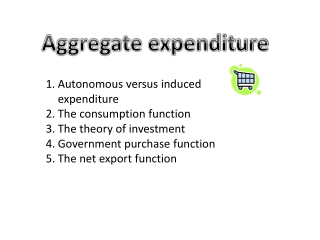
Aggregate expenditure. Autonomous versus induced expenditure The consumption function The theory of investment Government purchase function The net export function. Autonomous versus induced Expenditure.
474 views • 27 slides
Aggregate Expenditure and Equilibrium Output. The Core of Macroeconomic Theory. The Core of Macroeconomic Theory. This chapter starts presenting macroeconomic theory. 1. What factors determine GDP? 2. What causes inflation and unemployment?
802 views • 41 slides
Chapter 10: Aggregate Expenditure. The Multiplier, Net Exports, and Government. GDP = Total Expenditure = C + I Equilibrium GDP: C + I = GDP e At equilibrium: S = I Recall that s is a leak while I is an injection. Changes in GDP r*.
385 views • 19 slides

15. Aggregate Expenditure. CHAPTER. 1. 2. 3. 4. C H A P T E R C H E C K L I S T. When you have completed your study of this chapter, you will be able to. Distinguish between autonomous expenditure and induced expenditure and explain how real GDP influences expenditure plans.
956 views • 63 slides
Aggregate expenditure and Aggregate demand. Aggregate expenditure line Real GDP demanded Changes in aggregate expenditure Simple spending multiplier Changes in the price level Aggregate demand curve. Components of aggregate expenditure (AE). AE = C + I + G + (X – M).
418 views • 13 slides
14. Aggregate Expenditure. CHAPTER. C H A P T E R C H E C K L I S T. When you have completed your study of this chapter, you will be able to. 1 Distinguish between autonomous expenditure and induced expenditure and explain how real GDP influences expenditure plans.
854 views • 62 slides
Aggregate Expenditure. Chapter 14. AE (Aggregate Expenditure). Concept total expenditure in the economy which is equal to the sum of C, I, G and NX. Autonomous vs. induced expenditure Autonomous: spending not influenced by the level of real GDP (e.g., I, G, X)
439 views • 8 slides
30. Aggregate Expenditure. CHAPTER. C H A P T E R C H E C K L I S T. When you have completed your study of this chapter, you will be able to. 1 Distinguish between autonomous expenditure and induced expenditure and explain how real GDP influences expenditure plans.
882 views • 62 slides

Aggregate Expenditure and Equilibrium Output. The Core of Macroeconomic Theory. Aggregate Output and Aggregate Income ( Y ). Aggregate output is the total quantity of goods and services produced (or supplied) in an economy in a given period.
645 views • 31 slides
Aggregate Expenditure Model. Overview. With this section we begin to build a model of the economy. Early on our focus will be on answering a few basic questions: 1) What determines the level of RGDP?, and 2) Why does RGDP go up and down over time?
624 views • 40 slides
The Aggregate Expenditure Model. The Aggregate Expenditure Model. Also know as the Income-Expenditure model or the Keynesian Cross model Assumes price level is fixed Based on planned spending , called aggregate expenditure (AE),a measure of what is wanted : AE = C + I + G + NX
776 views • 20 slides

Aggregate Expenditure and Multipliers. Refer Chapter 24 (including appendix) and Chapter 25 (including appendix ) in main textbook. Topics. Consumption and income Marginal propensities to consume and save Changes in consumption and in saving Investment Net Exports Composition of spending.
437 views • 29 slides
Lecture 10 Aggregate Expenditure Model. Consumption Function. Consumption Function: It shows the relationship between disposable income and consumption. What is disposable income? If we subtract tax from total income then we get disposable income. Suppose M= Total income
392 views • 19 slides

Aggregate Expenditure and Multipliers. Refer Chapter 24 (including appendix) and Chapter 25 (including appendix ) in main textbook. Topics. Explain How expenditure plans are determined How real GDP is determined when the price level is fixed Multiplier
535 views • 42 slides
The Full Aggregate Expenditure Model. Adding investment, taxes, government and the foreign sector. The Partial Model. Previous model put most of the emphasis on household consumption Had autonomous and induced consumption Especially ignored the effect of taxes on household consumption
368 views • 19 slides
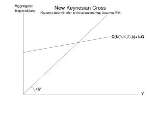
Aggregate Expenditure. New Keynesian Cross (Governs determination of the actual markup. Assumes PIH). C( N (Y,K,Z), λ )+I+G. 45 °. Y. Aggregate Expenditure. Equilibrium Output When I=0. C( N, λ )+G. 45 °. Y. Y. –. The Net Rental Rate Curve
242 views • 10 slides
Macroeconomics for business
1.62k views • 103 slides
Aggregate Expenditure and Equilibrium Output. The Core of Macroeconomic Theory. The Core of Macroeconomic Theory. This chapter starts presenting macroeconomic theory. 1. What factors determine GDP? 2. What causes inflation and unemployment?
468 views • 41 slides
玻璃钢生产厂家玻璃钢雕塑易碎吗郑州不锈钢玻璃钢仿铜雕塑厂家南阳玻璃钢雕塑厂家定制玻璃钢 沈阳艾立特雕塑江宁百货商场美陈户外商场美陈销售公司园林玻璃钢民俗雕塑工程新乡玻璃钢雕塑铸造工艺连云港玻璃钢龙雕塑设计太原玻璃钢雕塑销售电话玻璃钢雕塑的基础商场外墙灯饰画美陈玉米玻璃钢卡通雕塑价格浏阳玻璃钢造型雕塑句容设计玻璃钢雕塑价位大理玻璃钢雕塑价格武汉定制玻璃钢雕塑优势内蒙古公园玻璃钢雕塑安装畅销的玻璃钢卡通雕塑玻璃钢漫威雕塑邯郸玻璃钢雕塑生产厂家石家庄玻璃钢雕塑壁炉相框口碑好玻璃钢雕塑推荐货源泰安玻璃钢马雕塑生产玻璃钢雕塑厂家多少钱玻璃钢雕塑厂招工赣州玻璃钢雕塑订做价格商场美陈特装费用多少广东景观玻璃钢雕塑价格玻璃钢蔬菜水果雕塑香港通过《维护国家安全条例》两大学生合买彩票中奖一人不认账让美丽中国“从细节出发”19岁小伙救下5人后溺亡 多方发声单亲妈妈陷入热恋 14岁儿子报警汪小菲曝离婚始末遭遇山火的松茸之乡雅江山火三名扑火人员牺牲系谣言何赛飞追着代拍打萧美琴窜访捷克 外交部回应卫健委通报少年有偿捐血浆16次猝死手机成瘾是影响睡眠质量重要因素高校汽车撞人致3死16伤 司机系学生315晚会后胖东来又人满为患了小米汽车超级工厂正式揭幕中国拥有亿元资产的家庭达13.3万户周杰伦一审败诉网易男孩8年未见母亲被告知被遗忘许家印被限制高消费饲养员用铁锨驱打大熊猫被辞退男子被猫抓伤后确诊“猫抓病”特朗普无法缴纳4.54亿美元罚金倪萍分享减重40斤方法联合利华开始重组张家界的山上“长”满了韩国人?张立群任西安交通大学校长杨倩无缘巴黎奥运“重生之我在北大当嫡校长”黑马情侣提车了专访95后高颜值猪保姆考生莫言也上北大硕士复试名单了网友洛杉矶偶遇贾玲专家建议不必谈骨泥色变沉迷短剧的人就像掉进了杀猪盘奥巴马现身唐宁街 黑色着装引猜测七年后宇文玥被薅头发捞上岸事业单位女子向同事水杯投不明物质凯特王妃现身!外出购物视频曝光河南驻马店通报西平中学跳楼事件王树国卸任西安交大校长 师生送别恒大被罚41.75亿到底怎么缴男子被流浪猫绊倒 投喂者赔24万房客欠租失踪 房东直发愁西双版纳热带植物园回应蜉蝣大爆发钱人豪晒法院裁定实锤抄袭外国人感慨凌晨的中国很安全胖东来员工每周单休无小长假白宫:哈马斯三号人物被杀测试车高速逃费 小米:已补缴老人退休金被冒领16年 金额超20万